This post summarizes the historical milestones and evolution of the Attention and Transformer, which is one of the most important state-of-the-art machine learning models. It’s also a review material of the Deep Learning for Data Science lecture given by the professor Ziwei Liu.

Recurrent Neural Networks

The story of Transformer model begins with RNNs. In sequence-to-sequence learning, RNNs consist of an encoder and a decoder. In the encoder, the current hidden stat h_t is calculated from the previous hidden state h_t-1 and the current input x_t. After the encoder, two parameters are obtained to encapsulate the knowledge learned from the input sequence: an initial decoder state s_0 and a context vector c. In the decoder, each hidden state is calculated from the previous hidden state, the same context vector and the previous output token. Therefore, the calculation of output sequence is in series, depening on the previous output token.

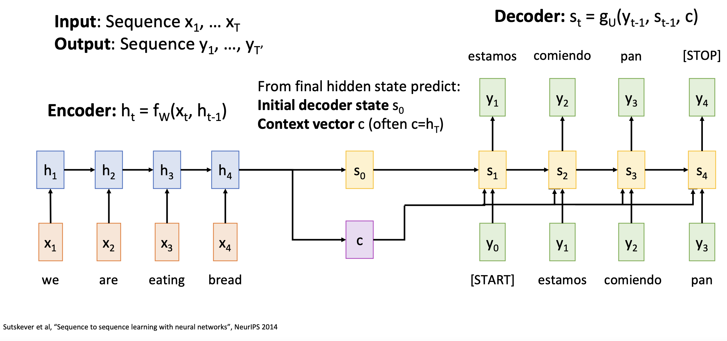
The problem with this RNN architecture lies in the fixed-size context vector, which becomes the bottleneck for learning long sequences. One idea to solve this issue is to use a new context vector at each step of decoder.

Recurrent Neural Networks and Attention

Attention introduces multiple context vectors into the decoder (one vector c per step). Each context vector attends to the relevent part in the input sequence. The context vector is computed as linear combination of hidden states with attention weights. The attion weights are obtained by the alignment (i.e., similarity) between the decoder state and each encoder hidden state through a softmax function.

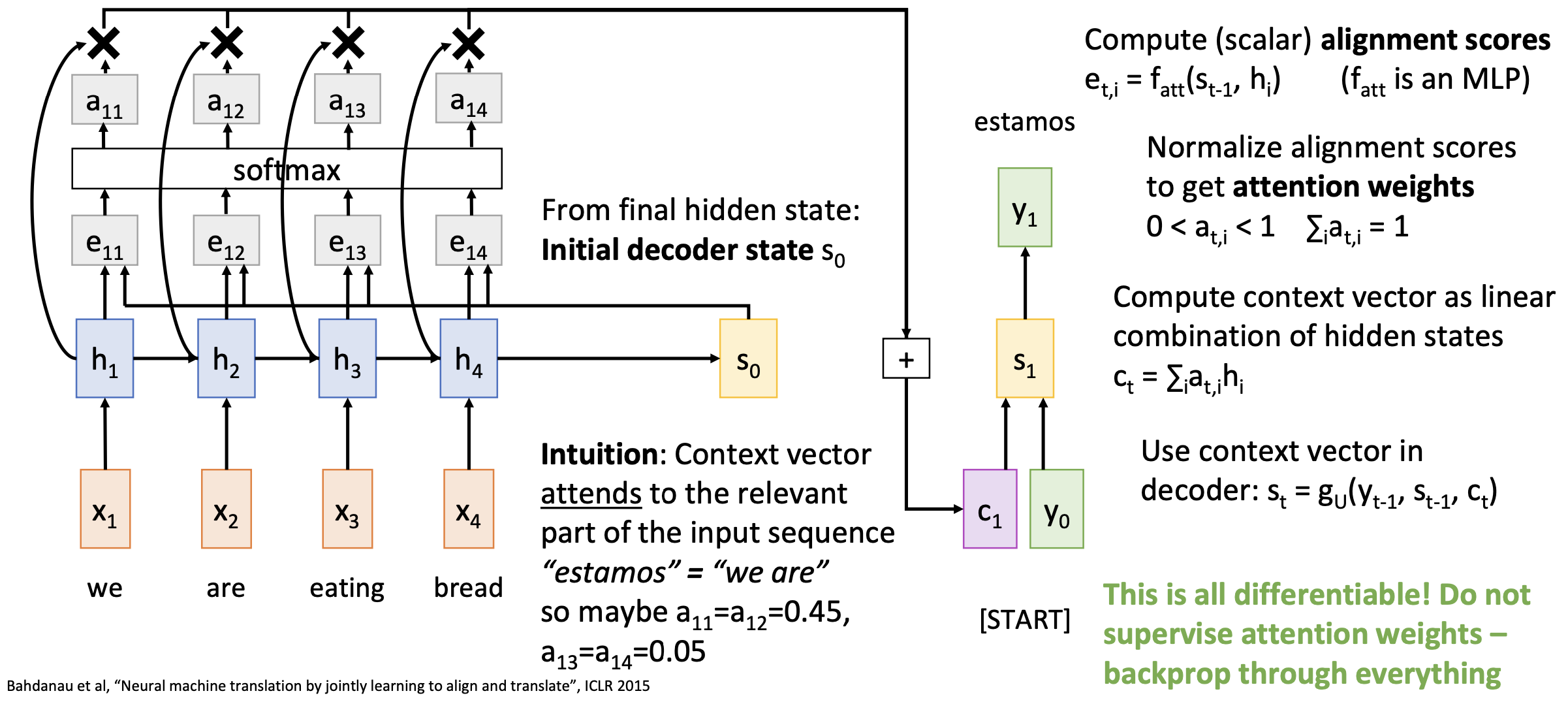
Use a different context vector in each timestep of decoder

• Input sequence not bottlenecked through single vector
• At each timestep of decoder, context vector “looks at” different parts of the input sequence

The decoder doesn’t use the fact that h_i form an ordered sequence – it just treats them as an unordered set {h_i}.

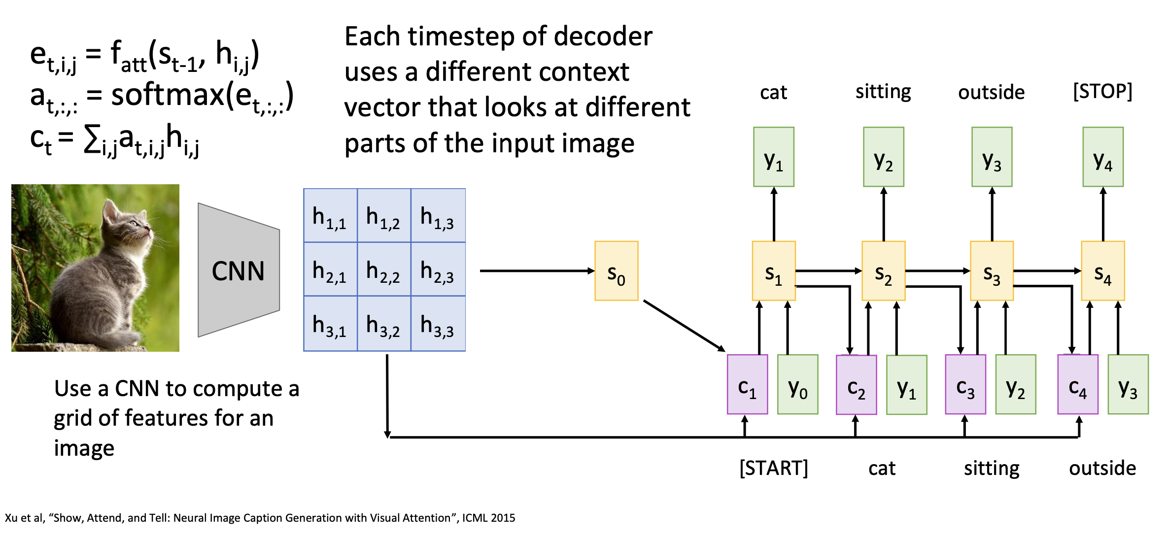
Image Captioning with RNNs and Attention

The input sequence and aligment score are 1-D vectors in the sequence-to-sequence learning. They can be also in 2-D like the case of image captioning. A pre-trained image encoder is used to extract feature matrix from the image. Each output word has a context vector attending to all values in the feature matrix.

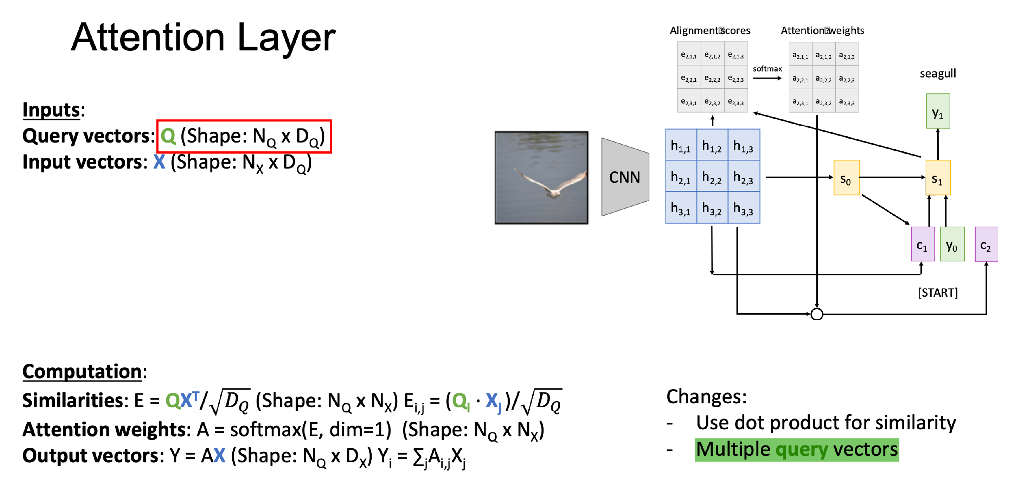
Attention Layer

In the next milestone, researchers work on including the RNN and Attention architecture into a single layer, called Attention Layer.

1. Query vector q is used as the same function of hidden state. Similarity score is measured between q and input X.
2. Dot-product is used for the similarity function to replace MLP.
3. Dot-product is scaled down by query dimension because large similarities will cause softmax to saturate and give vanishing gradients.
4. Stack the query vectors of all steps together into a query matrix Q.
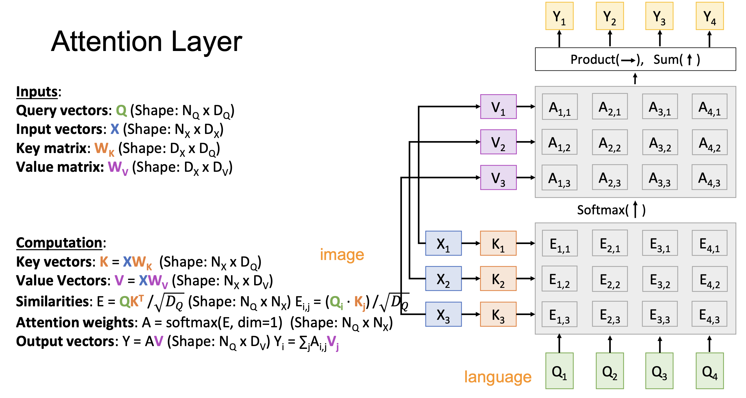
5. Increase the model complexity by adding key matrix and value matrix. Now the similarity is measured between query matrix Q and key matrix K. The output is obtained from the attention weights and the value matrix V, not directly from the input X.

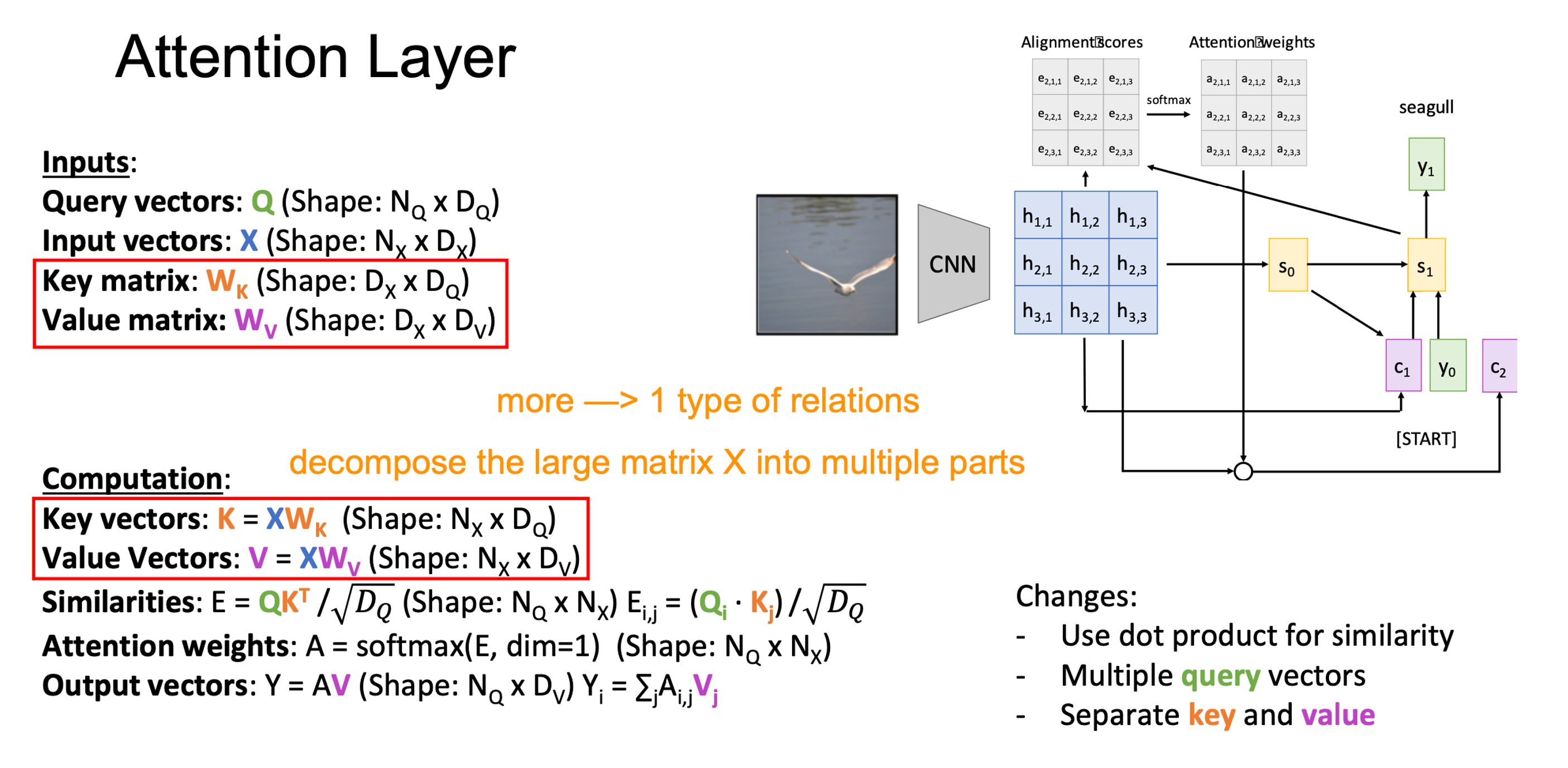
The final attention layer is formed as below.

Self-Attention Layer

The above cases deal with inputs with multi-modality (i.e., image and language sentence). Inputs Q (e.g., language) and X (e.g., image) are from different data sets. In the case where there is only one modal input, Q can be computed from X, which is called Self-Attention. As Q and K vectors are from the same input X, the attention is paid by a part of the input to another part of the input.

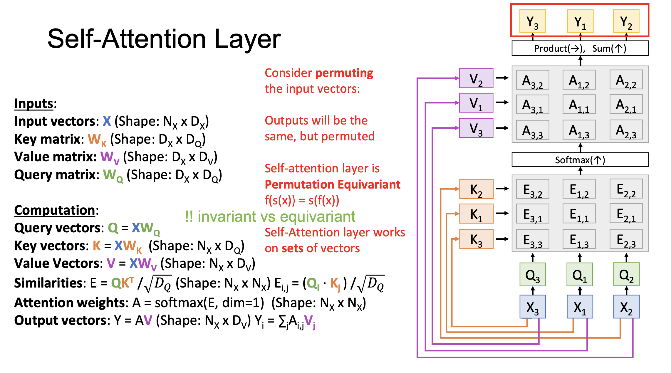
A key feature of Self-Attention is the Permutation Equivariant, which means when the order of inputs is changed, the outputs will be the same but permuted accordingly. Notably, it’s different from the Invariant, which refers to the characteristic that outputs don’t change along with the change of inputs.

Because Self-Attention doesn’t “know” the order of the vectors it is processing, a positional encoding E is concatenated with the input X. E can be a learned lookup table, or a fixed function.

Masked Self-Attention Layer

The mask is introduced into Self-Attention Layer to prevent vectors from “looking ahead” in the sequence. At each step, Q can only attend to K in the current and previous steps. Attention weight is set 0 between the former V and the latter V, for example, A_(1,2) is set to 0 and A_(2,1) is not.

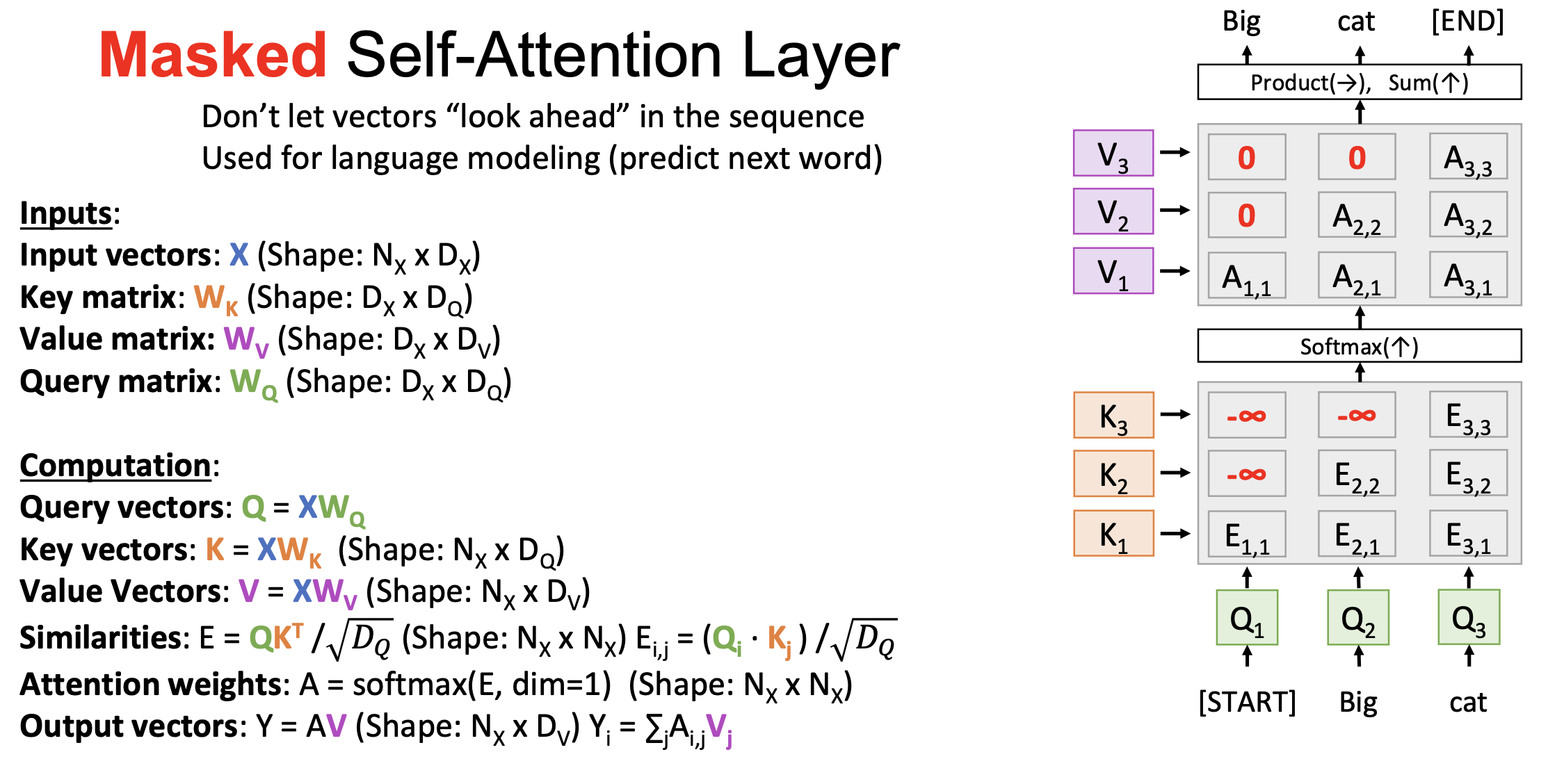
To learn different attention patterns at the same time, we can have multiple “Attention Heads” in parallel for query Q. Q dimension can be further spilt into independent parts (i.e., Heads H).

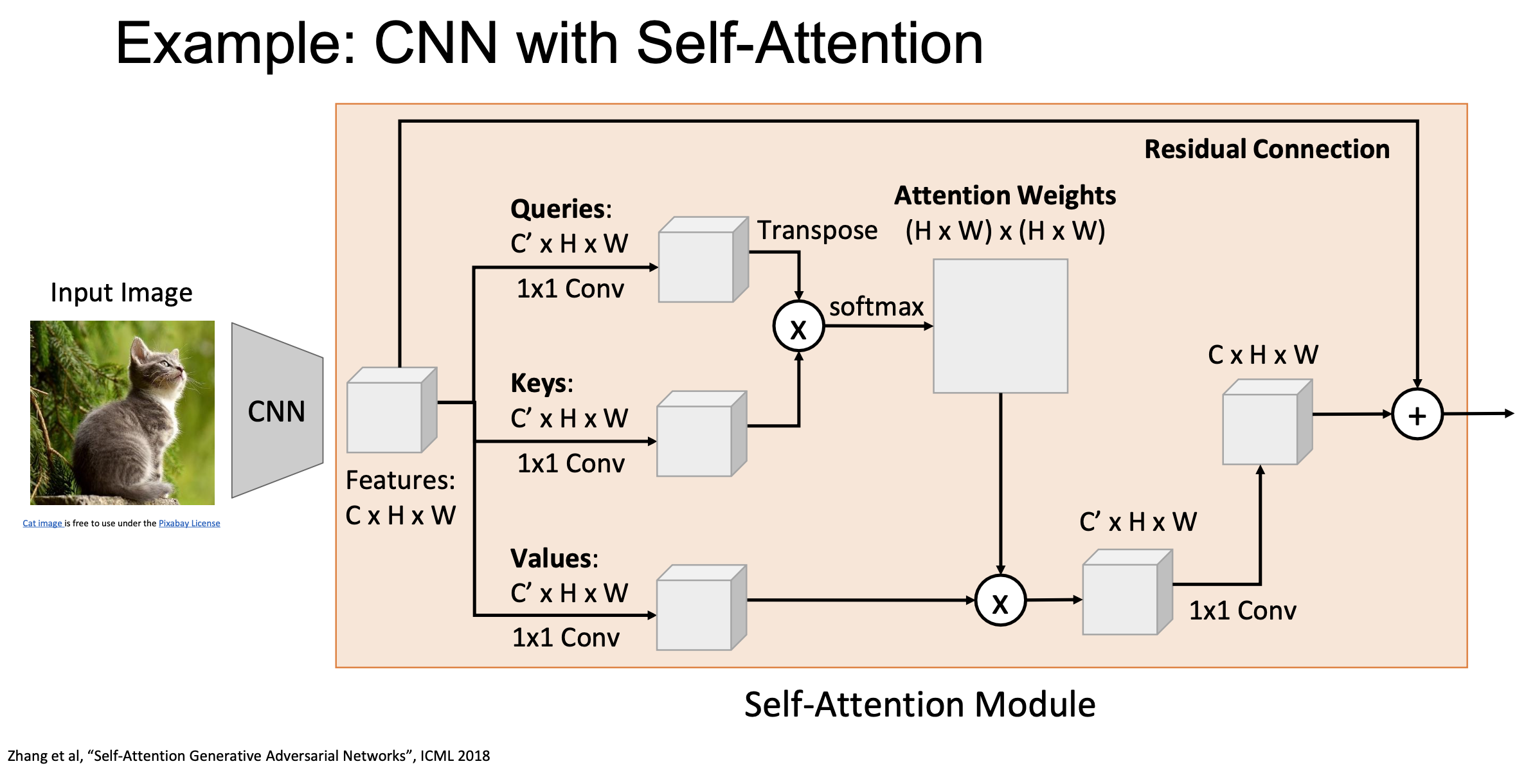
CNN with Self-Attention

Self-Attention architecture can be integrated into CNN. Instead of matrix multiplication, Query, Key and Value can be computed by applying 1x1 convolution to the input features. 1x1 convolution is handy to be used for changing channel dimension. An example Self-Attention Module is listed below.

Transformer

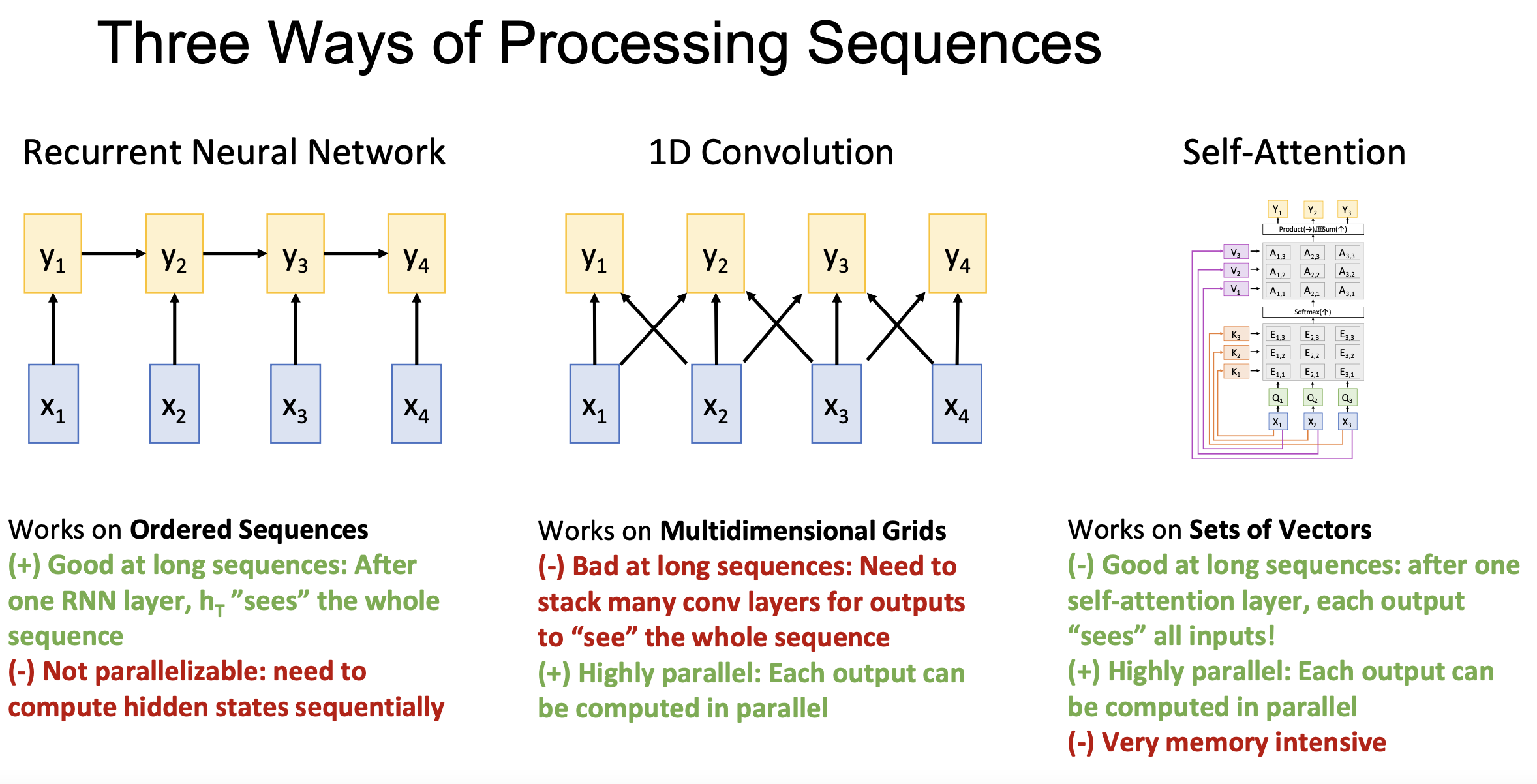
A comparion of three ways of sequence processing is shown.

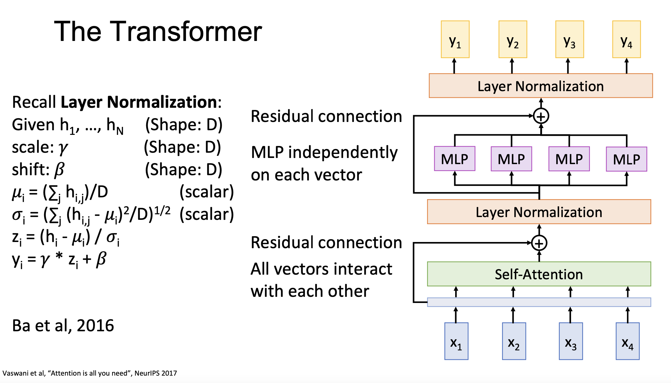
Finally, the Transformer block is constructed by Self-Attention, Residual Connection, Layer Normalization and MLP. Each input vector x has an independent MLP. Self-attention is the only interaction between vectors, which makes the transformer highly scalable and highly parallelizable.

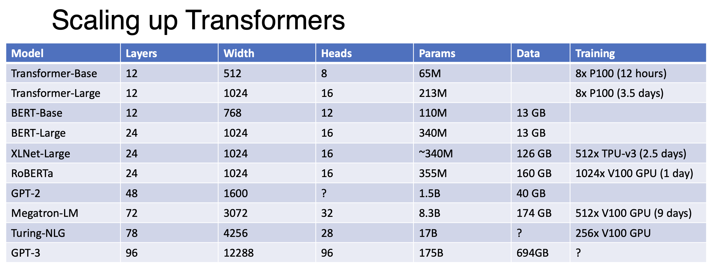
A Transformer is a sequence of transformer blocks. Pretraining and fine-tuning become the mainstream paradigm of language task workflow. Companies are working on larger datasets and deeper layers.