This post summarizes the key ideas in the field of image processing from the history. It is based on the NTU lecture CE7491 Image Processing given by the professors Cham Tat Jen and Loy Chen Change.

Classic Image Processing Techniques

Improve contrast

Contraset Stretching: present min gray level -> 0, max gray level -> 255, linear scale in-between

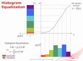
Histogram Equalization: flatten the gray-level histogram through a gray-level transformation, which uses a HE transfer function to map present pixel to new pixel. The pixel bin in the present histogram with high probability is converted to a larger bin in the new histogram with a fixed probability

Enhancement

Homomorphic Filtering: image = illumination (low frequencies) x reflectance (high frequencies), suppressing uneven illumination and increasing high-frequency components

Denoising

Median Filtering: remove impulse noise, also known as speckle or salt-and-pepper noise

Notch filters, Bandreject filters, Wiener filters: suppressing periodic interference noise

Smoothing

Gaussian Smoothing: filter is a 2D uniform variate normal density function

Sharpening

Laplacian Filter: filter is image derivatives, enhance edges only

High Boost Filtering: mix original image and Laplacian filtered image

Edge Detection

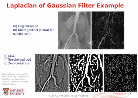
Sobel Filter: estimate the horizontal and vertical gradient magnitudes Gx and Gy separately

Laplacian of Gaussian Filter: edgel detection involves finding the zero-crossings in the output image, less sensitive to noise than using a Laplacian filter directly because of Gaussian smoothing

Canny Edge Detector:

1. Gaussian edge filtering: filter image by x and y 1st-order derivatives of a Gaussian
2. Non-maximal suppression: high gradient magnitudes are suppressed if they are not the local maxima in the gradient direction
3. Hysteresis (迟滞) thresholding: high and low thresholds, pixels with magnitudes between the two thresholds may be set to 1 if neighboring pixels perpendicular to edge gradient have been set to 1 (removing tiny noisy edges), also called neighbour support

Connect Edges

Hough Transform: maps a straight line in image space to a point in parameter space (Hough space), a point in image space corresponds to a sinusoidal curve in parameter space. Find the intersecting point in the parameter space, which is the connecting line in the image space.

Image Processing Concepts

Imaging Systems

Imaging devices have 3 key compoents:

• Apertune: control amount of light rays entering the device
• Optical system: focus light rays from 1 scene to converge at 1 point on the screen
• Screen: capture the image through photoreceptors

Field of View is the maximum angle of the scene observed by the camera.

Depth of Field is the range of depths that scene objects can be at, such hat they remain in acceptable focus simultaneously.

Pinhole cameras: Only 1 ray (the principal ray) from each scene point enters the pinhole, all of the scene at any depth is in focus.

Electric charge accumulates at each CCD cell and is proportional to (charge in CCD / CMOS cell can saturate)

• Irradiance (power of light falling on cell)
• Exposure time

Pixel: normally 1 unsigned byte integer (8 bits for 0-255 levels) Image Pixel Depth (gray-level resolution): the number of bits used to specify gray levels

Gray-Level Indexing: given reduced quantization, we can improve image quality through gray-level indexing. This involves using an indexed table with 2^n entries of the desired gray-levels specified to an arbitrary large number of bits (»n).

Dithering: Image dithering involves trading off spatial resolution for perceptual increase in pixel depth. Multiple neighboring pixels are used to synthesize in-between gray-levels via averaging in the human visual system.

Intensity

Point Processing: each pixel’s new gray-level does not depend on other pixel’s gray-level;

Spatial Filtering: each pixel’s new gray-level depends on current gray-level of neighbouring pixels;

Histogram Transfer: conserve the histogram count (number of pixels), i.e., pixel range * probability, map the present image hisogram to the new image histogram

Array Operation: arithmetic and logic operations with other images

• Masking
• Subtraction
• Averaging

Spatial Filtering: compute each pixel new gray-level based on the existing gray-levels of neighboring pixels (convolving), sometimes the filter h(x,y) is also known as the Point-Spread Function (PSF), since an input impulse becomes ‘spread out’

Nonlinear Filtering: using order statistics, e.g., median filter

Frequency

Analogous to 1D signals, 2D signals can be decomposed into sums of 2D sinusoidal components of the form

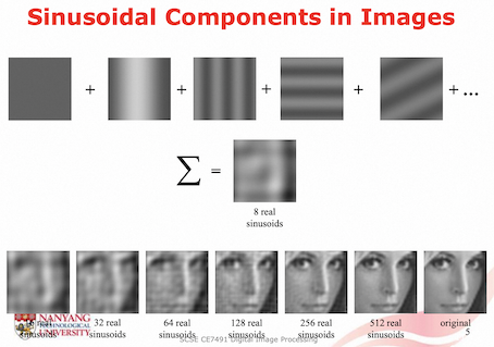
2D Discrete Fourier Transform (DFT) is a way of extracting key information about sinusoidal waves that make up an M x N image. It is like:

1. Turning a radio knob to scan different frequency channels
2. Measuring the response at each channel

2D DFT Output is a 2D index to sinusoidal waves, u=25, v=104 indexes to a wave of frequency, horizontal: 25/256 cycles/pixel, vertical: 104/256 cycles/pixel; contents of cell is a complex number, consisting of magnitude and phase

Original image f(x,y) -> DFT -> Frequency domain F(u,v)

Convolution Theorem: convolution of two spatial images is equivalent to multiplying the corresponding DFTs

Typical Framework for image processing in the frequency domain:

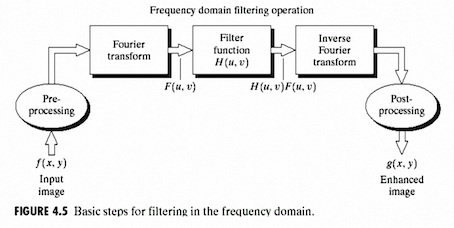
Filter Function H(u,v): we can design different filter to achieve different effects:

• Ideal Lowpass Filter (Cylindrical)
• Gaussian Lowpass Filter (variance sigma simultaneously controls both cutoff frequency as well as steepness of the cutoff)
• Butterworth Lowpass Filter (cutoff frequency and steepness are separately controled by two parameters)

Color

Light is electromagnetic (EM) radiation, EM waves are different simply because of their wavelengths. EM radiation can be characterized by a spectral power distribution (SPD), power (P) against wavelength (ν)

Color sensation is a simplified human representation (or summary) of incoming SPD. Different SPD’s can generate the same color sensation

Tristimulus Color Theory: a gamut of colors can be humanly perceived by physically adding 3 primary SPD’s in different amounts, any SPD can be primary – not limited to R, G, B. RGB color space is usually device-dependent, Standard RGB (sRGB) color space becoming popular, which are device-independent primaries

No set of 3 physically real primary SPD’s can reproduce all perceptible colors additively

Luminance defines approximately the brightness perception of different colors, Y = 0.2125 R + 0.7154 G + 0.0721 B

Chromaticity (色度) is the color attribute which is independent of luminance, colors with same ratio of tristimulus values have same chromaticity

HSI Color Space:

• Hue (色调): how similar is the color to the different primaries（不同色）
• Saturation (饱和度): how deep or ‘colorful’ the color is (i.e. how far the color is from gray)（色灰不灰）
• Intensity (亮度): refers to brightness of the color（色亮不亮）

Edge

Edgels: sharp and locally maximum gray-level gradient in one direction, small gray-level change in perpendicular direction

Ridges: located between parallel & near & sharp gradients in opposite directions

Sobel Filter: estimate the horizontal and vertical gradient magnitudes Gx and Gy separately

Laplacian of Gaussian Filter: edgel detection involves finding the zero-crossings in the output image, less sensitive to noise than using a Laplacian filter directly because of Gaussian smoothing

Advantages of Gaussian edge filtering:

• Robustness to noise
• Able to selectively detect edges at different scales

Hough Transformation groups straight image edges that belong to the same physical edge in the world. Edge points that lie on a common straight line in the image will have their corresponding curves intersecting at a common point in parameter space.

Image Restoration

Super-Resolution

Objectives:

• Increase the resolution of images
• Produce a detailed, realistic output image
• Be faithful to the low resolution input image

Multi image super-resolution combines information across frames and images. Need to address the mis-alignment problem

Single image super-resolution is inherently ill-posed since a multiplicity of solutions exist for any given low-resolution pixel. In other words, it is an underdetermined inverse problem, of which solution is not unique -> constraining the solution space by strong prior information

Sparse coding: a patch can be represented as a sparse linear combination of atoms. In training, learn low-resolution and high-resolution atom dictionaries. During inference, patches are encoded by a low-resolution dictionary, then multiplied by sparse coefficients to reconstruct high-resolution patches.

Weaknesses: sparse coding is computationally expensive to implement even at test time for finding the optimized encoding

SRCNN: first DL model, end-to-end between low- and high-resolution images, first upscales via bicubic interpolation

Peak signal-to-noise ratio (PSNR) is an expression for the ratio between the maximum possible value (power) of a signal and the power of distorting noise that affects the quality of its representation, but it doesn’t reflect human perception well

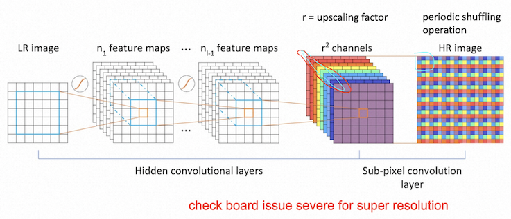
FSRCNN: no bicubic interpolation, dimensionality reduction via 1x1 conv filters (to change size of channels), dimensionality expansion with transposed convolution

Subpixel Convolution: Conv LR image to r^2 (r = upscaling factor), periodic shuffling values in each channel to form the HR image

Losses:

• Per-pixel loss (MSE)
• Perceptual loss (compare high-level representations from pretrained CNN)

Generative Adversarial Networks (GAN): 𝐷 (discrinimator) and 𝐺 (generator) play the following two-player minimax game with value function 𝑉(𝐺, 𝐷)

Prior for Restoration

Conditional Super-Resolution adds on categorical prior (classification mask) with LR images; only concatenating mask in the input layer doesn’t work well since prior tends to be forgotten across deep networks; Spatial Feature Transform (SFT) modulates the feature maps in each layers. Restoration quality decreases with fewer SFT layers.

Deep Generative Prior: GAN trained on large-scale natural images for richer priors beyond a single image, as GAN is a good approximator for natural image manifold.

Face Restoration:

• Reduce the uncertainty and ambiguity of LQ-to-HQ mapping.
• Complement high-quality details lost in the LQ inputs.
• Be robust against heavy degradations while maintaining identity consistency.

Face Priors:

1. Geometric Prior: the average magnitude of residual maps between HR and the bicubic interpolation of LR, high-frequency prior (e.g., face edge) indicates the location with high-frequency details
2. Exemplars: reference on similar faces
3. Generative Prior: GAN as latent bank

CodeFormer learns discrete codebook prior in a small proxy space to reduce the uncertainty and ambiguity of restoration mapping by, while providing rich visual atoms for generating high-quality faces

VAE models latent vector by a combination of the mean and standard deviation of the output of the convolutions

VQVAE uses vector quantisation to obtain a discrete latent representation. It differs from VAEs in two key ways: the encoder network outputs discrete, rather than continuous; and the prior is learnt via codebook rather than static (the posteriors and priors in VAEs are assumed normally distributed with diagonal covariance)

VQGAN:

1. Codebook Learning: get the chosen codebook vector as close to the encoder output as possible; getting the encoder output to commit as much as possible to its closest codebook vector
2. Codebook Lookup Transformer
3. Controllable Feature Transformation: Continuous Transitions between Image Quality and Fidelity

Transformers

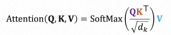
Attention is a mechanism that a model can learn to make predictions by selectively attending to a given set of data.

Self-attention is a type of attention mechanism where the model makes prediction for one part of a data sample using other parts of the observations about the same sample.

Rather than only computing the attention once, the multi-head mechanism runs through the scaled dot-product attention multiple times in parallel. Multi-head attention allows the model to jointly attend to information from different representation subspaces at different positions.

Batch Normalization is found unstable in Transformers, Layer Normalization works well with RNN and now being used in Transformers

Gaussian Error Linear Units (GELU) can be thought of as a smoother ReLU

Encoder-Decoder Attention layer works just like multiheaded self-attention, except it creates its Queries matrix from the layer below it, and takes the Keys and Values matrix from the output of the encoder stack.

ViT has much less image-specific inductive bias than CNNs.

1. Inductive bias in CNN: Locality, Two-dimensional neighborhood structure, Translation equivariance
2. Inductive bias in ViT: Only MLP layers are local and translationally equivariant. Self-attention layer is global. Two dimensional neighborhood is used sparingly, only at the beginning where we cut image into patches and learnable position embedding

ViT overfits the ImageNet task due to its lack of inbuilt knowledge about images.

ViT having more uniform representations, with greater similarity between lower and higher layers. With NO large-scale pre-training (just training on ImageNet), ViT has much lower performance than CNN

Swin Transformer

• Perform local self-attention thus having linear computational complexity with respect to the number of tokens
• Shifted window between consecutive self-attention layers to allow connections
• Flexibility to model at various scales with hierarchical representation

Diffusion Models

Encoder: mix the input data with noise until only noise remains. With enough steps, the conditional distribution and marginal distribution of the final latent variable both become the standard normal distribution. The encoding process is prespecified, all the learned parameters are in the decoder.

Decoder: a series of networks are trained to map backward between each adjacent pair of latent variables, removing noise at each stage. The loss function encourages each network to invert the corresponding encoder step. After training, new examples are generated by sampling noise vectors and passing them through the decoder.

Diffusion kernel: generating samples z_t sequentially is time-consuming when t is large, using close-form expression directly draw samples z_t given initial data point x

We approximate the reverse distributions as normal distributions, using neural network to compute the mean of the normal distribution in the estimated mapping from z_t to the preceding latent variable z_t-1

Loss function for each diffusion time step consists of reconstruction term (with original image) and residual term (between target and predicted z_t-1)

The loss function is modified so that the model aims to predict the noise that was mixed with the original data example to create the current variable. Works better in practice.

Denoising Diffusion Implicit Models (DDIM): One of the major drawbacks of diffusion models is that they take a long time to train and sample from. DDIM defines the forward process is defined only on a sub-sequence of time steps. This allows a reverse process that skips time steps and hence makes sampling much more efficient; good samples can be created with 50 time steps when the forward process is no longer stochastic. This is much faster than before but still slower than most other generative models.

Conditional generation: adding an extra term into the update step during the reverse process to bias the denoising update toward that class, which is the gradient of the log likelihood of an auxiliary classifier model. Weakness: this classifier must be trained on noisy data so it is generally not possible to plug in a pre-trained classifier

Latent Diffusion Model, e.g., Stable Diffusion, projects the original image data to a smaller latent space using a conventional autoencoder (e.g., VAE) and then runs the diffusion process in this smaller space. Advantages: reduce the dimensionality of the training data for the diffusion process, allow other data types (text, graphs, etc.) to be described by diffusion model.

Image Synthesis

Desired Properties of Latent Representations:

1. Compact: low-dimensional, or sparse, distributed, 1 latent dimension related to many output instances -> bottlenecking
2. Invariant: unaffected by factors we don’t care about, e.g. noise, variations to ignore -> data augmentation with unwanted variations
3. Disentangled: relevant factors of variation are separated into different subspaces / dimensions -> Partition latent factors into different spaces

Intended separation by bottlenecking (~compaction)

• Latent code: variable input parameters
• Decoder weights: invariant attributes for reconstruction

Modelling Probability Distributions:

• Parametric methods (e.g., Gaussian)
• Cluster based (e.g., histogram)
• Kernel density estimation
• Distribution as samples

KDE involves placing a kernel (a smooth, symmetric, and usually bell-shaped) at each data point. The kernel represents the shape of the probability density around that point. The individual kernels are then summed or combined to create a smooth estimate of the underlying distribution. This is done for each data point in the dataset.

Evidence Lower Bound (ELBO) consists of reconstruction term and KL divergence term.