This is the assignment of NTU CE7455: Deep Learning For Natural Language Processing by Prof. Luu Anh Tuan. In this assignment, I have implemented and analyzed different deep learning models for sentiment classification. Detailed report refers to here.

Data Preparation

TorchText Field is define how the data should be processed. In its parameters, the spaCy tokenizer is used to split the string into discrete “tokens”. The tokenizer_language tells torchtext which spaCy model to use. LabelField is used to process the sentiment.

import torch
from torchtext import data

SEED = 1234

torch.manual_seed(SEED)
torch.backends.cudnn.deterministic = True

TEXT = data.Field(tokenize = 'spacy',
                  tokenizer_language = 'en_core_web_sm',
                  include_lengths = True,
                  pad_first=True)
LABEL = data.LabelField(dtype = torch.float)

The IMDb dataset is downloaded and split into train (25,000)/test (25,000) objects. The IMDb dataset consists of 50,000 movie reviews, each marked as being a positive or negative review. An example is as below:

{‘text’: [‘As’, ‘part’, ‘of’, ‘our’, ‘late’, ‘1950s’, ‘vocabulary’, ‘,’, ‘we’, ‘well’, ‘knew’, ‘the’, ‘Ponderosa’, ‘,’, ‘Little’, ‘Joe’, ‘,’, ‘Hoss’, ‘,’, ‘Ben’, ‘Cartwright’, ‘,’, ‘etc’, ‘.’, ‘on’, ‘that’, ‘great’, ‘show’, ‘”’, ‘Bonanza’, ‘.’, ‘“<br’, ‘/><br’, ‘/>It’, ‘came’, ‘Saturday’, ‘night’, ‘and’, ‘everyone’, ‘was’, ‘glued’, ‘to’, ‘the’, ‘television’, ‘set’, ‘.’, ‘This’, ‘was’, ‘a’, ‘real’, ‘show’, ‘depicting’, ‘family’, ‘values’, ‘.’, ‘There’, ‘may’, ‘have’, ‘been’, ‘a’, ‘weekly’, ‘crisis’, ‘,’, ‘but’, ‘it’, ‘was’, ‘the’, ‘strong’, ‘family’, ‘atmosphere’, ‘that’, ‘pulled’, ‘everyone’, ‘together.<br’, ‘/><br’, ‘/>Lorne’, ‘Greene’, ‘was’, ‘dominant’, ‘as’, ‘the’, ‘patriarch’, ‘of’, ‘the’, ‘family’, ‘.’, ‘His’, ‘words’, ‘depicted’, ‘wisdom’, ‘.’, ‘We’, ‘often’, ‘were’, ‘left’, ‘to’, ‘wonder’, ‘that’, ‘Ben’, ‘Cartwright’, ‘,’, ‘a’, ‘widower’, ‘,’, ‘must’, ‘have’, ‘been’, ‘the’, ‘best’, ‘of’, ‘husbands’, ‘to’, ‘that’, ‘poor’, ‘wife’, ‘of’, ‘his’, ‘who’, ‘had’, ‘died’, ‘.’, ‘He’, ‘reared’, ‘wonderful’, ‘sons.<br’, ‘/><br’, ‘/>Naturally’, ‘,’, ‘we’, ‘all’, ‘wondered’, ‘why’, ‘Pernell’, ‘Roberts’, ‘left’, ‘the’, ‘show’, ‘.’, ‘The’, ‘show’, ‘was’, ‘a’, ‘gold’, ‘mine’, ‘and’, ‘Roberts’, ‘surrendered’, ‘loads’, ‘of’, ‘money’, ‘when’, ‘he’, ‘departed’, ‘.’, ‘His’, ‘career’, ‘never’, ‘took’, ‘off’, ‘as’, ‘he’, ‘was’, ‘associated’, ‘as’, ‘a’, ‘Cartwright’, ‘son’, ‘.’, ‘He’, ‘should’, ‘have’, ‘tried’, ‘to’, ‘get’, ‘back’, ‘into’, ‘the’, ‘series’, ‘.’, ‘He’, ‘certainly’, ‘lost’, ‘a’, ‘bonanza’, ‘by’, ‘dropping’, ‘out’, ‘.’], ‘label’: ‘pos’}

30% of train data is split out as evaluation data, where random_state is defined by the random seed to ensure that we get the same train/validation split each time.

A vocabulary is a effectively a look up table where every unique word in data set has a corresponding index (an integer). The number of unique words in our training set is over 100,000, which means that our one-hot vectors will have over 100,000 dimensions! This will make training slow and possibly won’t fit onto your GPU (if you’re using one). There are two ways effectively cut down our vocabulary, we can either only take the top $n$ most common words or ignore words that appear less than $m$ times. Here, we do the former, only keeping the top 25,000 words. The rest words are replaced by the <unk> token, e.g., “This film is great and I <unk> it”. Apart from that, there is another special token, called <pad>.

When we feed sentences into our model, we feed a batch of them at a time, i.e. more than one at a time, and all sentences in the batch need to be the same size. Thus, to ensure each sentence in the batch is the same size, any shorter than the longest within the batch are padded.

The most frequent words are, TEXT.vocab.freqs.most_common(10):

[(‘the’, 203031), (‘,’, 192565), (‘.’, 166394), (‘and’, 109412), (‘a’, 109239), (‘of’, 100823), (‘to’, 93911), (‘is’, 76237), (‘in’, 61332), (‘I’, 54701)]

The methods .stoi (string to int) or .itos (int to string) are handy to check words, TEXT.vocab.itos[:10]:

[‘', '', 'the', ',', '.', 'and', 'a', 'of', 'to', 'is']

The final step of preparing the data is creating the iterators. We iterate over these in the training/evaluation loop, and they return a batch of examples (indexed and converted into tensors) at each iteration. We’ll use a BucketIterator which is a special type of iterator that will return a batch of examples where each example is of a similar length, minimizing the amount of padding per example.

Model Building

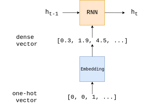
The embedding layer is used to transform our sparse one-hot vector (sparse as most of the elements are 0) into a dense embedding vector (dense as the dimensionality is a lot smaller and all the elements are real numbers). This embedding layer is simply a single fully connected layer. As well as reducing the dimensionality of the input to the RNN, there is the theory that words which have similar impact on the sentiment of the review are mapped close together in this dense vector space.

Finally, the linear layer takes the final hidden state and feeds it through a fully connected layer, transforming it to the correct output dimension.

import torch.nn as nn

class RNN(nn.Module):
    def __init__(self, input_dim, embedding_dim, hidden_dim, output_dim):
        
        super().__init__()
        
        self.embedding = nn.Embedding(input_dim, embedding_dim)
        
        self.rnn = nn.RNN(embedding_dim, hidden_dim)
        
        self.fc = nn.Linear(hidden_dim, output_dim)
        
    def forward(self, text, text_lengths):
        #text = [sent len, batch size]

        embedded = self.embedding(text)
        #embedded = [sent len, batch size, emb dim]
        
        output, hidden = self.rnn(embedded)
        #output = [sent len, batch size, hid dim]
        #hidden = [1, batch size, hid dim]
        
        #assert torch.equal(output[-1,:,:], hidden.squeeze(0))
        
        return self.fc(hidden.squeeze(0))

A batch in train_iterator has a dimension of [sentence length, batch size]. PyTorch conveniently stores a one-hot vector as it’s index value, i.e. the tensor representing a sentence is just a tensor of the indexes for each token in that sentence. The act of converting a list of tokens into a list of indexes is commonly called numericalizing. The input batch is then passed through the embedding layer to get embedded, which gives us a dense vector representation of our sentences. embedded is a tensor of size [sentence length, batch size, embedding dim].

embedded is then fed into the RNN. In some frameworks you must feed the initial hidden state, h_0 , into the RNN, however in PyTorch, if no initial hidden state is passed as an argument it defaults to a tensor of all zeros.

The RNN returns 2 tensors, output of size [sentence length, batch size, hidden dim] and hidden of size [1, batch size, hidden dim]. output is the concatenation of the hidden state from every time step, whereas hidden is simply the final hidden state. We verify this using the assert statement. Note the squeeze method, which is used to remove a dimension of size 1.

assert torch.equal(output[-1,:,:], hidden.squeeze(0))

• The input dimension is the dimension of the one-hot vectors, which is equal to the vocabulary size.
• The embedding dimension is the size of the dense word vectors. This is usually around 50-250 dimensions, but depends on the size of the vocabulary.
• The hidden dimension is the size of the hidden states. This is usually around 100-500 dimensions, but also depends on factors such as on the vocabulary size, the size of the dense vectors and the complexity of the task.
• The output dimension is usually the number of classes, however in the case of only 2 classes the output value is between 0 and 1 and thus can be 1-dimensional, i.e. a single scalar real number.

This function tells how many trainable parameters the model has (the numel() function is used to get the total number of elements in a tensor):

def count_parameters(model):
    return sum(p.numel() for p in model.parameters() if p.requires_grad)

print(f'The model has {count_parameters(model):,} trainable parameters')

Model Training

Optimizer is the algorithm used to to update the parameters of the model. Different optimizers are tested including SGD, Adam and Adagrad. The learning rate is set to decide how much we’ll change the parameters by when we do a parameter update.

Criterion defines the loss function used in the training. For classification, we can use binary cross entropy with logits. Our model currently outputs an unbound real number. As our labels are either 0 or 1, we want to restrict the predictions to a number between 0 and 1. We do this using the sigmoid or logit functions. The BCEWithLogitsLoss criterion carries out both the sigmoid and the binary cross entropy functions.

A train function is created to iterate over all examples, one batch at a time. model.train() function is used to put the model in “training mode”, which turns on dropout and batch normalization.

For each batch, we first zero the gradients. Each parameter in a model has a grad attribute which stores the gradient calculated by the criterion. PyTorch does not automatically remove (or “zero”) the gradients calculated from the last gradient calculation, so they must be manually zeroed.

We then feed the batch of sentences, batch.text, into the model. The squeeze is needed as the predictions are initially size [batch size, 1], and we need to remove the dimension of size 1 as PyTorch expects the predictions input to our criterion function to be of size [batch size].

The loss and accuracy are then calculated using our predictions and the labels, batch.label, with the loss being averaged over all examples in the batch. We calculate the gradient of each parameter with loss.backward(), and then update the parameters using the gradients and optimizer algorithm with optimizer.step().

TorchText sets tensors to be LongTensors by default, however our criterion expects both inputs to be FloatTensors.

Model Evaluation

model.eval() puts the model in “evaluation mode”, this turns off dropout and batch normalization. Again, we are not using them in this model, but it is good practice to include them.

No gradients are calculated on PyTorch operations inside the with no_grad() block. This causes less memory to be used and speeds up computation.

The rest of the function is the same as train, with the removal of optimizer.zero_grad(), loss.backward() and optimizer.step(), as we do not update the model’s parameters when evaluating.

We then train the model through multiple epochs, an epoch being a complete pass through all examples in the training and validation sets.

At each epoch, if the validation loss is the best we have seen so far, we’ll save the parameters of the model and then after training has finished we’ll use that model on the test set.